Decision Trees for Classification
Before we begin to analyze and dissect the functional structure of Decision Trees (also referred to as Classification Trees), it is critical to motivate its applications in the machine learning world.
In general, many machine learning models tend to be obscure in how exactly they learn from data. Although the algorithms behind these models are well studied and have a vast literature, choices made within the learning process are still not well defined for a human examiner. In contrast, decision trees are extremely interpretable as the choices made by the algorithm are conditionally formulated.
Conditionally formulated, in the context of Decision Trees, means that the algorithm can be described as a series of if-else statements that test different attributes of an instance to ultimately produce a classification.
Assume we have trained a Decision Tree as follows:
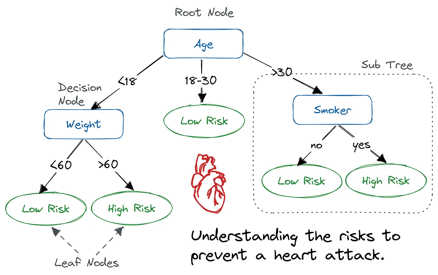
The tree structure of the model allows us to characterize a few key traits:
- Each non-leaf node tests the value of a given attribute
- Each leaf node represents a classification
- Each branch of a node, i, indicates one possible value of the attribute tested in i
- The path from the root node to a leaf node defines a classification rule
Let us assume we want to classify a new instance:
\[x = \{Age: 34, Weight: 70 \, \text{kgs}, Smoker: no\}\]
The root node is where we always begin the traversal. We go through each branch of Age and check to see if Age satisfies the condition. Observe that Age satisfies the last branch (from the left) because \(34 > 30\). Then we test if x is a smoker. Our data indicates that x is in fact not a smoker and so we classify x as Low Risk.
One thing to note is that we never tested Weight for this instance — this is ok! This is a common possibility of a trained Decision Tree.
Training
Thus far we have discussed how to use a trained Decision Tree to make classifications. But, in order to truly understand the implications that underly these models, we should also take a dive into the actual training process.
Find the best attribute
Imagine we have a dataset with m attributes for each instance. The first step would be to find the best attribute to test. To do this, we need to define a criterion that will allow us to measure how informative testing on a particular attribute will be.
There are many variations of criterions, but for the purposes of simplicity, we will focus on Information Gain.
Before we introduce Information Gain, it is crucial that we deterministically represent what exactly information of a dataset is. In the context of Decision Trees, information of a dataset is more commonly referred to as the entropy of that dataset. To better illustrate what entropy is, let us utilize an example:
Dataset = {
  "Amanda": "iPhone",
  "John": "iPhone",
  "Sam": "Blackberry",
  "Robert": "iPhone",
  "Ruby": "Blackberry",
  "Shirley": "iPhone"
}
There are two unique classes — iPhone and Blackberry — for which we need to find the probabilities for. This step is a simple counting problem:
\[P(\text{iPhone}) = \frac{\# \text{ of instances with class iPhone}}{\# \text{ of instances}} = \frac{4}{6} = \tfrac{2}{3}\]
\[P(\text{Blackberry}) = \frac{2}{6} = \tfrac{1}{3}\]
From here we use the formula for information gain provided below.
\[I(p_1, p_2, ... , p_n) = -p_1 \log(p_1) - p_2 \log(p_2) - \dots - p_n \log(p_n)\]
In our case \(n=2\), because there are only two unique classes and \(p_1 = \tfrac{2}{3}\) while \(p_2 = \tfrac{1}{3}\). Thus, we end up with an entropy of:
\[I\left(\tfrac{2}{3}, \tfrac{1}{3}\right) = -\tfrac{2}{3} \log\left(\tfrac{2}{3}\right) - \tfrac{1}{3} \log\left(\tfrac{1}{3}\right)\]
We can now start to form an intuition as to what exactly entropy is telling us about the dataset.
Entropy tells us how heterogeneous our dataset is.
Note that heterogeneous means “how mixed up is our data — particularly the class labels.” So, when making predictions about a certain class, we would like the data to be as homogeneous as possible.
Imagine having 5 apples and 5 oranges in a bag (very heterogeneous, not homogeneous). Would you be able to confidently predict what fruit you will get if you blindly choose? Probably not.
Alternatively, if we had 9 apples and 1 orange in a bag (very homogeneous, not too heterogeneous), it becomes easier to predict that apples would be the fruit you will get.
Consequently:
- Lower entropy → more homogeneous → more informative the dataset is about a particular class.
How exactly does this tie into Information Gain?
The idea is straightforward: we want to measure how much information we would gain if we were to split on a certain attribute. Once again, let us use an example.
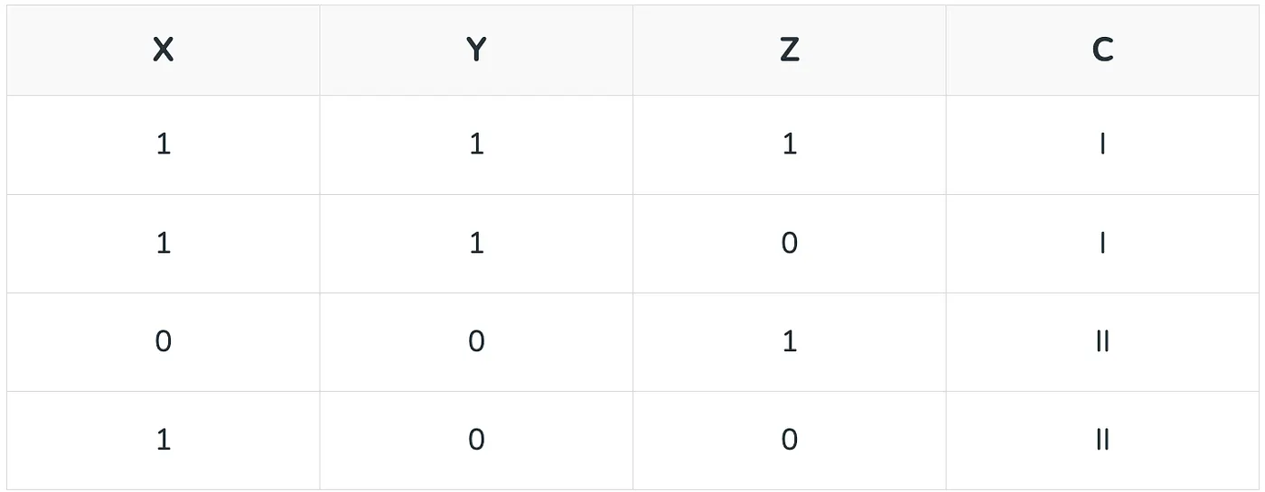
Imagine we choose to split on the attribute X. We would split into two branches — one for \((X = 1)\) and \((X = 0)\) each.
Within the branch \((X = 1)\) we will have 2 instances of class I and one instance of class II. Thus, our entropy will be:
\[I[X](\tfrac{2}{3}, \tfrac{1}{3}) = -\tfrac{2}{3} \log\left(\tfrac{2}{3}\right) - \tfrac{1}{3} \log\left(\tfrac{1}{3}\right)\]
The information gain will consequently be defined as the original entropy prior to the split minus the entropy after the split:
\[IG = I[\text{original}] - I[X]\]
Ok, thus far, we have defined what a decision tree is and also presented a criterion to measure information gained from splitting based on an attribute.
But how do we actually utilize this? On a high level, we recurse the dataset:
- Start with the initial dataset, find the optimal attribute (in our case, optimal means the attribute with the highest information gain).
- Split on the attribute, \(X\), and create sub-branches, one for each value \(X\) can take.
- Each sub-branch will have a partitioned version of the original dataset \(D\). Use the partitioned dataset, \(PD\), as the new dataset!
- Now recurse! That’s it.
Of course, there are still some concerns that I haven’t and will not cover for the purposes of this article. Some of the most pressing concerns are:
- How do we split on numerical attributes? The method I have described is for categorical attributes where branches are representative of the categories an attribute can take.
- When to stop recursing? There are many stopping criterions that you should definitely spend time analyzing.
- Are there any other criterions I can use as a metric for information? Yes! Feel free to explore them.